LIDAR for Autonomous System Design: Object Classification or Object Detection?
November 13, 2020
Story
The promise of a fully autonomous tomorrow no longer seems like a pipe dream.
The promise of a fully autonomous tomorrow no longer seems like a pipe dream. Today, the questions around autonomy center on the underlying technologies and the advancements needed to make autonomy a reality. Light detection and ranging (LIDAR) has become one of the most discussed technologies supporting the shift to autonomous applications, but many questions remain. LIDAR systems with ranges greater than 100 m and 0.1° of angular resolution continue to dominate autonomous driving technology headlines.
However, not all autonomous applications require this level of performance. Applications such as valet park assist and street sweeping are two such examples. There are plenty of depth sensing technologies that enable these applications, such as radio detection and ranging (radar), stereo vision, ultrasonic detection and ranging, and LIDAR. However, each of these sensors has a unique trade-off between performance, form factor, and cost. Ultrasonic devices are the most affordable, but are limited in range, resolution, and dependability. Radar is much improved in range and dependability, but it also has angular resolution limitations, while stereo vision can have a large computational overhead and limitations in accuracy, if not calibrated properly. Thoughtful LIDAR system design helps bridge these gaps with precision depth sensing, fine angular resolution, and low complexity processing, even at long ranges. However, LIDAR systems are typically viewed as bulky and costly, which needn’t be the case.
LIDAR system design begins with identifying the smallest object the system needs to detect, the reflectivity of that object, and how far away that object is positioned. This will define the system’s angular resolution. From that, the minimum achievable signal-to-noise ratio (SNR) can be calculated, which is the true/false positive or negative detection criteria needed to detect the object.
Understanding the perception environment and amount of information necessary to make the appropriate design trade-offs enables the development of the optimal solution relative to both cost and performance. For example, consider an autonomous automobile traveling down a road at 100 kph (~27 mph) as compared to an autonomous robot moving around a pedestrian space or warehouse at 6 kph. In the high-speed case, it may be relevant to consider not only the vehicle moving at 100 kph, but also another vehicle driving at the same speed in the opposite direction. To a perception system, this equates to an object approaching at a relative speed of 200 kph. For a LIDAR sensor that detects objects at a maximum distance of 200 m, the vehicles would have closed the distance between them by 25% in just one second. It should be emphasized that the vehicle’s velocity (or the nonlinear closing speed to the object), stopping distance, and dynamics involved in performing evasive maneuvers are complexities unique to every situation. In general, it can be stated that longer range LIDAR systems are needed for high speed applications.
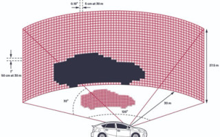
Resolution is another important system characteristic of LIDAR system design. Fine angular resolution enables the LIDAR system to receive return signals in multiple pixels from a single object. As shown in Figure 1, angular resolution of 1° translates to pixels 3.5 m per side at a range of 200 m. Pixels this size are larger than many of the objects that need to be detected, which presents several challenges. For one, spatial averaging is often used to improve SNR and detectability, but with only one pixel per object, it is not an option. Further, even if detected, it becomes impossible to predict the size of an object. A piece of road debris, an animal, a traffic sign, and a motorcycle are all typically smaller than 3.5 m. By contrast, a system with 0.1° angular resolution has pixels 10 times smaller and should measure approximately five adjacent returns on an average width car at 200 m distance. The dimensions of most cars are typically wider than they are tall; thus, this system could likely distinguish a car from a motorcycle.
Detecting whether an object can be safely driven over requires much finer resolution in elevation as compared to azimuth. Now imagine how different the requirements of an autonomous vacuum robot could be as it travels slowly and needs to detect narrow but tall objects such as table legs.
With distance and speed of travel defined, as well as the object and subsequent performance requirements established, the architecture of the LIDAR system design can be determined (see the example LIDAR system in Figure 2). There are a multitude of choices to be made, such as scanning vs. flash, or direct time of flight (ToF) vs. waveform digitization, but their trade-offs are beyond the scope of this article.

(Figure 1. A LIDAR system with 32 vertical channels scanning the environment horizontally at an angular resolution of 1°.)

(Figure 2. Discrete components of a LIDAR system.)

(Figure 3. Analog Devices AD-FMCLIDAR1-EBZ LIDAR development solution system architecture.)
Range, or depth, precision is related to the ADC sample rate. Range precision allows the system to know exactly how far away an object is, which can be critical in use cases that necessitate close-quarters movement, such as parking or warehouse logistics. Additionally, the change in range over time can be used to calculate velocity, and this use case will often require even better range precision. With a simple thresholding algorithm such as direct ToF, the range precision achievable is 15 cm for a 1 ns sample period—that is, with a 1 GSPS ADC. This is calculated as c(dt/2), where c is the speed of light and dt is the ADC sample period. Given that an ADC is included, however, more sophisticated techniques, such as interpolation, can be used to improve range precision. As an estimate, the range precision can be improved by roughly the square root of the SNR. One of the highest performance algorithms for processing data is a matched filter, which maximizes SNR, followed by interpolation to yield the best range precision.
The AD-FMCLIDAR1-EBZ is a high performance LIDAR prototyping platform, and is a 905 nm pulsed direct ToF LIDAR development kit. This system enables quick prototyping for robotics, drones, and agricultural and construction equipment, as well as ADAS/AV with a 1D static flash configuration. The components selected for this reference design are targeted at a long range, pulsed LIDAR application. The system is designed with a 905 nm laser source driven by the ADP3634, a high speed, dual 4 A MOSFET. It also includes a First Sensor 16-channel APD array powered by the LT8331, a programmable power supply, to generate the APD supply voltage. There are multiple 4-channel LTC6561 TIAs for their low noise and high bandwidth, and an AD9094 1 GSPS, 8-bit ADC, which has the lowest power consumption per channel at 435 mW/channel. There will continue to be a need to increase bandwidth and sampling rates, which help with overall higher system frame rates and improved range precision. At the same time, it is important to minimize power consumption, as less heat dissipation simplifies thermal/mechanical design and permits a reduced form factor.
Another tool to aid in LIDAR system design, the EVAL-ADAL6110-16 is a highly configurable evaluation system. It provides a simplified, yet configurable, 2D flash LIDAR depth sensor for applications needing real-time (65 Hz) object detection/tracking, such as collision avoidance, altitude monitoring, and soft landing.

(Figure 4. EVAL-ADAL6110-16 LIDAR evaluation module using the integrated 16-channel ADAL6110-16.)
The optics used in the reference design result in a field of view (FOV) of 37° (azimuth) by 5.7° (elevation). With a linear array of 16 pixels oriented in azimuth, the pixel size at 20 m is comparable to an average adult, 0.8 m (azimuth) × 2 m (elevation). As discussed previously, different applications may need different optical configurations. If the existing optics do not meet the application needs, the printed circuit board can be easily removed from the housing and incorporated into a new optical configuration.
The evaluation system is built around ADI’s ADAL6110-16, which is a low power, 16-channel, integrated LIDAR signal processor (LSP). The device provides the timing control for illuminating the field of interest, the timing to sample the received waveform, and the ability to digitize the captured waveform. The ADAL6110-16’s integration of sensitive analog nodes reduces the noise floor, enabling the system to capture very low signal returns as opposed to implementing the same signal chain with discrete components of similar design parameters where the rms noise can dominate the design. Further, the integrated signal chain allows for LIDAR system designs to reduce size, weight, and power consumption.
The system software enables fast uptime to take measurements and begin working with a ranging system. It is fully standalone and operates off a single 5 V supply over USB, and can also be easily integrated into an autonomous system with provided robot OS (ROS) drivers. Users need only create a connector for the header to interface with their robot or vehicle and communicate via one of the four available communication protocols: SPI, USB, CAN, or RS-232. The reference design can also be modified for different receiver and emitter technologies.
As previously mentioned, the EVAL-ADAL6110-16 reference design’s receiver technology can be modified to create different configurations as shown in Figure 5 through Figure 7. The EVAL-ADAL6110-16 is supplied with a Hamamatsu S8558 16-element photodiode array. The size of the pixel at varying distances displayed in Table 1 is based on the effective pixel size, which is 0.8 mm × 2 mm, along with the 20 mm focal length lens. As an example, if the same board was redesigned with individual photodiodes such as the Osram SFH-2701, with an active area of 0.6 mm × 0.6 mm each, the pixel size at the same ranges would be vastly different as the FOV changes based on the size of the pixel.
Table 1. Receiver Size and Optics Used in the EVAL-ADAL6110-16 and a Potential Pixel Arrangement If the Receiver Was Changed to SFH-2701


(Figure 5. Dimensions of the Hamamatsu S8558 PIN photodiode array.)
For example, let’s review the S8558 with its 16 pixels arranged in a line with each
pixel dimension: 2 mm × 0.8 mm.

(Figure 6. A basic calculation of the angular resolution using simple optics.)
After selecting a 20 mm focal length lens, the vertical and horizontal FOV per pixel can be calculated by using basic trigonometry, as shown in Figure 6. Of course, lens selection can involve additional, more complex considerations, such as aberration correction and field curvature. For lower resolution systems such as this, however, straightforward calculations are often sufficient.
The 1 × 16 pixel FOV selected can be used in applications such as object detection and collision avoidance for autonomous vehicles and autonomous ground vehicles, or to enable simultaneous localization and mapping (SLAM) for robots in constrained environments such as warehouses.
A unique application involves configuring the array in a 4 × 4 grid to detect objects around a system. This application under development will be mounted on motor coaches and RVs as a safety bubble around the vehicle that can warn the driver if distracted individuals are walking within bus proximity. The system could detect the direction in which an individual is walking and warn the driver to act by stopping the vehicle or alerting the pedestrian with their horn in order to prevent hitting the individual or bicyclist.
Remember, not every application calls for a 0.1° angular resolution and 100 m range. Take time to consider what the application truly needs from a LIDAR system design, then clearly define the key criteria, such as object size, reflectivity, distance to object, and the speed at which the autonomous system is traveling. This will inform the component selection for a balanced design of optimal performance and cost relative to the functionality the system needs, ultimately increasing the likelihood of a successful design the first time around.

(Figure 7. Various optical implementations of a LIDAR system that can help enhance application safety.)
About the Author
Sarven Ipek joined ADI in 2006. During his tenure at Analog Devices, Sarven has attained a breadth of experience in failure analysis, design, characterization, product engineering, and project and program management. Sarven is currently a marketing manager within the Autonomous Transportation and Safety Group's LIDAR division at Analog Devices in Wilmington, MA. He has a Bachelor of Science in electrical and computer engineering, as well as a Master of Science in electrical engineering with a concentration in communication systems and signal processing, both from Northeastern University. He can be reached at [email protected].
About the Author
Ron Kapusta is an Analog Devices Fellow and holds B.S. and M.Eng. degrees from the Massachusetts Institute of Technology. Upon graduating in 2002, he joined Analog Devices, designing data converters and sensor interface circuits for digital imaging systems. In 2014, Ron shifted focus to automotive technologies, working on electronics, photonics, and signal processing for LIDAR sensors. Ron has also been involved in program committees for several IEEE conferences. He can be reached at [email protected].