Consider the creation of a frequency domain filter supporting between 1 million and 16 million points on current FPGA architectures with sample rates from 120 million to 240 million samples per second. The example looks at design decision options for a 2 million-point single-precision frequency domain filter using OpenCL.

Such a filter translates its input into the frequency domain using a multimillion-point one-dimensional (1D) FFT, multiplies each frequency and phase component by a separate user-provided value, and then translates the result back into the time domain with an inverse FFT. The overall target performance requirement of the whole system is 150 million samples per second (MSPS) for a 2 million-point sample size on a current-generation FPGA with two DDR3 external memory banks. Inputs and outputs come over 10 gigabit Ethernet (GbE) directly into the FPGA.

The design uses the Altera SDK for OpenCL FPGA compiler targeting a BittWare S5-PCIe-HQ board with a Stratix V GSD8 FPGA. OpenCL, instead of a lower-level language, is used for two reasons:

1. The first reason is that designing multimillion-point filters requires building a complicated yet highly efficient external memory system. With lower-level design tools, creating individual blocks such as an on-chip FFT or a corner-turn is relatively easy (especially because every FPGA vendor already provides libraries containing such blocks). However, creating the external memory system would normally require a lot of HDL work. This situation can be especially challenging, as we will see later, because the configuration of the overall system is unknown at the very beginning.
2. The second reason for choosing OpenCL is host-level control over the FPGA logic. For this design, it is clear from the start that two full copies of multimillion point FFT cores will not fit on a single device, so a single data set will have to pass over the FPGA logic at least twice before producing the final output. Coordinating such sharing while also allowing features such as dynamically changing data set size, multiplication coefficients, and even completely changing FPGA functionality for something else is best left to a CPU.

Using the OpenCL compiler for FPGAs solves both of these challenges as it builds a customized and highly efficient external memory system while allowing fine-grained control over the FPGA logic.

On-chip FFT

For this design, it’s assumed that we already have an FFT core that can handle data sizes that fully fit on an FPGA (referred to as “on-chip FFT”), as every FPGA vendor provides such cores. Such a core is parameterizable in at least the following ways:

• Data type (fixed or single-precision floating point)
• Number of points to process (N)
• Number of points to process in parallel (POINTS)
• Dynamic support for changing the number of points to process

Given such an on-chip FFT core, building the overall system requires two steps: First, building an FFT core that can handle multimillion points, and second, stitching two such cores together with complex multiplication between them to create the whole system.

Multimillion-point FFT

The classic way to implement an FFT with external storage is the six-step algorithm shown in Figure 1 that treats a single, one-dimensional data set as two-dimensional (2M = 2K x 1K)[1].

 

 

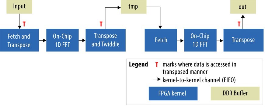
The six-step algorithm shows both the separate computation kernels and external memory buffers. The “Fetch” kernel reads data from external memory, optionally transposing it, and outputs it into a channel (also known as a “pipe” in OpenCL 2.0 nomenclature). In hardware, a channel is implemented as a FIFO with compiler-calculated depth. An “on-chip 1D FFT” is an unmodified vendor’s FFT core, taking input and producing a bit-reversed output using channels. “Transpose” always transposes the data it reads from its input channel, optionally multiplying it by special twiddle factors, and writes outputs in natural order to external memory.

As shown in the diagram, the data is sent over Fetch ➝ 1D FFT ➝ Transpose (F1T) pipeline twice to produce final output. This gives us our first important design choice: Either have one copy of the F1T pipeline to save area, or two copies for a higher possible throughput.

Initial prototyping of this algorithm is done in an emulator to ensure that address manipulation for transpositions and twiddle factors is correct. An emulator compiles OpenCL kernels to x86-64 binary code that can be run on a development machine without an FPGA. Going from emulator to hardware compile is a painless step, as functionally correct code in the emulator became functionally correct code in the hardware so no simulation is needed.

The only aspect that has to be modified, for performance and area reasons, is the local memory system used by the Fetch and Transpose kernels. Efficient transposition requires buffering POINTS columns/rows of data in local memory. The OpenCL compiler analyzes all accesses to local memory in the OpenCL code and creates a custom on-chip memory system optimized for that code. In the case of POINTS=4, the original transposition kernels had four writes and four reads. An on-chip RAM block, double-pumped, can service at most four separate requests with at most two of these being writes. To support four writes and four reads, on-chip memory needs to be both duplicated and contain request arbitration logic, which causes area bloat and performance loss. However, the write pattern can be changed to make all four writes consecutive. These four writes were grouped by the OpenCL compiler into a single, wide write, giving only five accesses to the local memory system: one write and four reads. With that change, the compiler automatically builds a much smaller five-ported memory system that could service all five requests on every clock cycle without stalling.

Once the design is compiled to hardware, it‘s time to measure performance. With a single copy of the F1T pipeline on the FPGA, we measure 217 MSPS with POINTS=4 and 457 MSPS with POINTS=8 for a 4 million-point FFT[2]. The POINTS=8 version used twice as many on-chip Block RAMs, and two copies in this configuration will not fit. This gives us the first design dimension to explore – the number of points to process in parallel versus area.

Full-filter design

Now that we have a multimillion point FFT, we are ready to put the whole design together. Simply stitching two off-chip FFTs gives us the logical view of the whole pipeline in Figure 2.

 

 

Besides duplicating a single off-chip FFT computation pipeline, the following parts are added to the system:

1. Complex multiplication in the frequency domain is absorbed into a third F1T block. The coef buffer is holding two million complex multiplication coefficients.
2. I/O in and I/O out kernels are added to realistically model the additional load of 10 GbE channels on external memory. With these kernels we can continue purely software-based development and leave Ethernet channel integration until after the core computation pipeline is fully optimized. The I/O in kernel generates a single sample every clock cycle, and I/O out consumes a single sample every clock cycle.

As experiments with off-chip FFT showed, we can fit only two F1T blocks, and only with POINTS=4. Therefore, the data has to pass through the hardware twice for full computation. That gives us an overall system throughput of only 120 MSPS for 2 million points, below our target of 150 MSPS. However, by reducing the data size to 1 million points, we are able to fit a POINTS=8 version and get throughput of 198 MSPS. That shows that there is still performance to be had, if only we can make a POINTS=8 version fit for 2 million points.

Picking an optimized structure of the full pipeline in Figure 2 is the next step in the overall design process. The first improvement we can make is to remove tmp3 buffer. Both sides access it in the same way (transposed write and read), and therefore the second and third F1T blocks can be connected directly by a channel. This requires making the Transpose kernel either write its output to external memory or into a channel, and a similar change for Fetch. Such a change is dynamically controlled by the host, so a single physical instance of Fetch can be used. Note that this changes our connectivity to external memory, but this is something we don’t have to worry about at all because the OpenCL compiler always generates an efficient custom external memory interconnect for our system.

A further improvement would be to move the second transpose “T” from writing to tmp1 to reading from tmp1 (the data in tmp1 will be stored differently but the net effect is the same). This eliminates the need for one local memory buffer used by transpositions. Even though this change is not hard to implement, we decide to forgo it in lieu of a more radical idea.

Our original transposition implementation is done in two stages:

First all the required data is loaded into local memory and then read from local memory using transposed addresses. To efficiently utilize such a pipeline, the OpenCL compiler automatically double-buffers the local memory system. This way, the loading part of the pipeline can load the data into one copy while the reading part can read previous data sets from another copy.

This automatic double buffering is the right thing to do for our transposition algorithm, but it’s expensive. Instead, we rewrite the transposition kernels to be in-place. Such a kernel only needs only a single buffer and supports reading and writing multiple data points at the same time (but we’ll leave a detailed description of this transposition kernel for another time).

With these changes we are able to fit a 2 million-point FFT in a POINTS=8 configuration and achieve 164 MSPS throughput.

Scheduling

Only two copies of F1T could fit, but Figure 3 shows how the data flow can be scheduled to fully utilize the pipeline. Notice that in a steady state, the pipeline alternates between processing two and three data sets at a time without additional buffers. This scheduling is controlled by the host program running on a CPU and verified using the Dynamic Profiler tool.

 

 

Buffer allocation

In an OpenCL system the host program controls which DDR bank contains which buffers. Since a DDR bank is most efficient when it’s either read from or written to, but not both, we can split the five buffers among two DDR banks as follows:

• DDR bank #0 gets input and tmp2
• DDR bank #1 gets tmp1, coef, and out

Assigning a buffer to a DDR bank is a one-line change in the OpenCL host program. The compiler and the underlying platform take care of the rest. Given such automation, we can experiment on 2-DDR and 4-DDR boards to find the best mapping of buffers to banks for each board.

Conclusion

This article describes how to design a 2 million-point frequency domain filter using the Altera OpenCL SDK for FPGAs. All functional verification was done using software-style emulation, and every single hardware compile worked correctly. We did not open a hardware simulator and never worried about timing closure.

References:

[1] Bailey, D.H. “FFTs in external of hierarchical memory.” Proceedings of Supercomputing’89 (SC89), pp. 234-242.

[2] “FFT (1D) Off-Chip Design Example.” Altera Corporation. www.altera.com/support/support-resources/design-examples/design-software/opencl/fft-1d-offchip.html.

Dmitry Denisenko is a senior software engineer at Altera Corporation.

Mykhailo Popryaga is a software engineer at Altera Corporation.

Altera Corporation www.altera.com LinkedIn Facebook