
Chances and challenges for machine learning in highly automated driving, part 2: Theoretical background
August 01, 2018
Story

Part two defines the theoretical background of machine learning technology, as well as the types of neural networks available to automotive developers.
In part one of this three-part series, the authors investigate the drivers behind and potential applications of machine learning technology in highly automated driving scenarios. Part two defines the theoretical background of machine learning technology, as well as the types of neural networks available to automotive developers. Part three evaluates these options in the context of functional safety requirements.
Machine learning can be defined as a set of algorithms that facilitate predictions based on past learning.
In a machine learning algorithm, the input data is organized as data points. Each data point consists of features that describe the represented data. For example, size and speed are features that can differentiate a car from a bicycle on the street. Both the size and the speed of a car are usually higher than those of a bicycle. The goal of the machine learning methodology is to convert the input data into a meaningful output, such as classifying the input data into car and non-car data points or objects. The input is usually written as vector x, composed from several data points. The output is written as y.
Two- or three-dimensional input data can be illustrated and viewed in a so-called feature space, where each data point in x is plotted with respect to its features. Figure 8 (a) shows a simplified example of a two-dimensional feature space that describes the car and non-car objects.
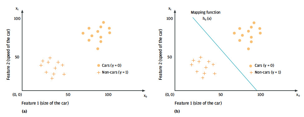
A so-called learned mapping function or model,h_θ (x), gives the difference between the feature vectors (e.g., the classification into car and non-car data points). The structure of the model ranges from a simple linear function, such as the line dividing car and non-car objects in Figure 8 (a), to a complex non-linear neural network. The goal of the learning methodology is to determine the values of the θ- coefficients, which represent the parameters of the model from the available input data. The output of the mapping function is the algorithm’s prediction of what the input data describes.
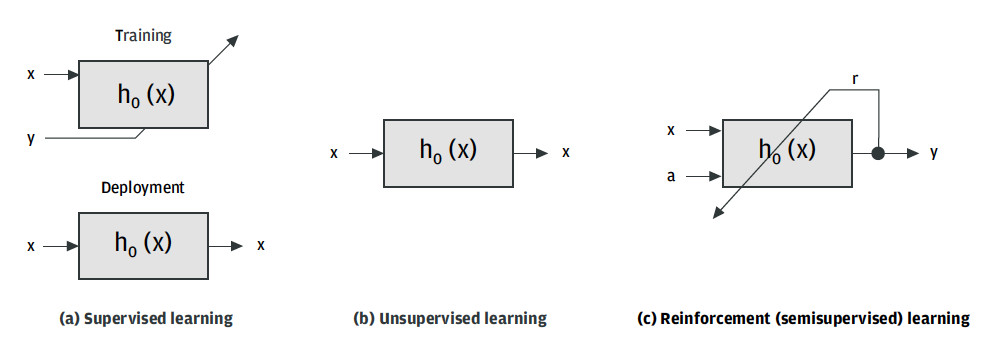
Machine learning methods can be classified according to how the mapping function is learned (Figure 9). There are three possibilities:
- Supervised learning – The mapping function is calculated from training data pairs where the output,
y, known in advance, is given to the learning algorithm separately during the training phase. The model can be deployed into the target application once its parameters have been computed. Its output – when it receives an unknown data point – will be the predicted value ofy. - Unsupervised learning – In this case there are no feature-label pairs available during the training phase, in contrast to supervised learning. The input to the learning algorithm consists only of unlabeled data points. The goal of this machine learning methodology is to deduce labels for the input features,
x, directly from their distribution in the feature space. - Reinforcement (semi-supervised) learning – The training data has no labels in this case, either, but the model is constructed to facilitate an interaction with its environment through a set of actions. The mapping function maps the state of the environment, which is given by the input data to actions. A reward signal indicates the performance of an action on a certain state of the environment. The learning algorithm reinforces the action when the signal indicates a positive influence. The algorithm will discourage the specific action or state of the environment if a negative influence is recognized.
The deep learning revolution
The so-called deep learning paradigm has revolutionized the machine learning field in recent years. Deep learning made a huge impact on the machine learning community by solving challenges that previously could not be tackled with traditional pattern recognition approaches (LeCun et al. 2015). The introduction of deep learning has dramatically improved the precision of systems designed for visual recognition, object detection, speech recognition, anomaly detection, or genomics. The key aspect of deep learning is that the features used to interpret the data are learned automatically from the training data instead of being manually crafted by an engineer.
Until now, the main challenge in constructing a good pattern recognition algorithm has been the manual engineering of the hand-crafted feature vector for classification, such as the local binary patterns used in an earlier version of the traffic sign recognition system as described in part 1. The emergence of deep learning has replaced manual engineering of the feature vectors with learning algorithms that can discover significant features in the raw input data automatically.
Architecturally, a deep learning system is made up from several layers of non-linear units, which can transform the raw input data into higher levels of abstraction. Each layer maps the output of the previous layer into a more complex representation that is suitable for regression or classification tasks. This learning is usually performed on a deep neural network that is trained by the use of a back-propagation algorithm. This algorithm iteratively adapts the parameters or weights of the network in order to mimic the input training data. The network thus has learned a complex non-linear mapping function of the input data points by the end of the training.
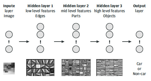
Figure 10 shows a symbolic representation of a deep neural network that is trained to recognize cars in images. The input layer represents the raw input pixels. Hidden layer 1 usually mimics the presence or absence of edges in certain locations and orientations of the image. The second hidden layer models object parts using the edges calculated in the previous layer. The third hidden layer builds an abstract representation of the modeled objects, which, in our case, is the way a car is imaged. The output layer calculates the probability that a given image contains a car, based on the high level features of the third hidden layer.
Different network architectures result from the way that the units and layers of a neural network are distributed. The so-called perceptron is the simplest, consisting of a single output neuron. A large number of neural network flavors can be obtained by building on the perceptron. Each of these networks is more suited to a specific application than others. Figure 11 shows three of the most common neural network architectures out of the many that have been created in recent years.
A deep feed-forward neural network (Figure 11a) is a structure in which the neurons between two neighboring layers are fully interconnected and the information flow is in one direction only, from the input to the output of the system. These networks are useful as general-purpose classifiers and are used as the basis for all other types of deep neural systems.
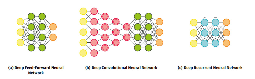
The deep convolutional neural network (Figure 11b) changed the way that visual perception methods are developed. Such networks are composed of alternate convolutional and pooling layers that learn object features automatically by generalization from the input data. These learned features are passed on to a fully interconnected feed-forward network for classification. This type of convolutional network is the basis of the car detection architecture shown in Figure 10 and the use cases described in part 1.
While deep convolutional networks are crucial to visual recognition, deep recurrent neural networks (Figure 11c) are essential for natural language processing. The information in such architectures is time-dependent due to the self-recursive connections between the neurons in the hidden layers. The output of the network can vary depending on the order in which data is fed into the network. For example, if the word "cat" is fed in before the word "mouse," a certain output is obtained. Now, if the input order changes, the output order may change, too.
Types of machine learning algorithms
Although deep neural networks are among the most often used solutions in complex machine learning challenges, there are various other types of machine learning algorithms available. Table 1 classifies them according to their nature (continuous or discrete) and training type (supervised or unsupervised).
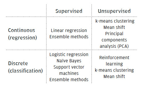
Machine learning estimators can be classified roughly according to their output value or training methodology. The algorithm is classed as a regression estimator if the latter estimates a continuous value function y (i.e., a continuous output). The machine learning algorithm is called a classifier when its output is a discrete variable ? R
y ? {0,1,…,q}. The traffic sign detection and recognition system described in part 1 is an implementation of this type of algorithm.
Anomaly detection is one special application of unsupervised learning. The goal here is to identify outliers or anomalies in the data set. The outliers are defined as feature vectors that have different properties compared to the feature vectors commonly encountered in the application. In other words, they occupy a different position in the feature space.
Table 1 also lists some popular machine learning algorithms. These are briefly explained below.
- Linear regression is a regression method used to fit a line, a plane, or a hyperplane to a dataset. The fitted model is a linear function that can be used to make predictions on the real value function
y. - Logistic regression is the discrete counterpart of the linear regression method, in which the predicted real value given by the mapping function is converted to a probability output that denotes membership of the input data point to a certain class.
- Naïve Bayes classifiers are a set of machine learning methods built on the basis of Bayes' theorem, which makes the assumption that each feature is independent of the other features.
- Support vector machines (SVM) are designed to calculate the separation between classes using so-called margins. The margins are computed to be as wide as possible in order to separate the classes as clearly as possible.
- Ensemble methods, such as decision trees, random forests, or AdaBoost combine a set of base classifiers, sometimes called “weak” learners, with the purpose of obtaining a “strong” classifier.
- Neural networks are machine learning algorithms in which the regression or classification problem is solved by a set of interconnected units called neurons. In essence, a neural network tries to mimic the function of the human brain.
- k-means clustering is a method used for grouping together features that have common properties, i.e., they are close to each other in the feature space. k-means iteratively groups common features into spherical clusters based on the given number of clusters to group.
- Mean-shift is also a data clustering technique, which is more general and robust with respect to outliers. As opposed to k-means, mean-shift requires only one tuning parameter (the search window size) and does not assume a spherical prior shape for the data clusters.
- Principal components analysis (PCA) is a data dimensionality reduction technique that transforms a set of possibly correlated features into a set of linearly uncorrelated variables named principal components. The principal components are arranged in order of variance. The first component has the highest variation; the second has the next variation below this, and so on.
Part three evaluates these machine learning algorithms in the context of functional safety requirements.
Associate Professor Sorin Mihai Grigorescu received his Dipl.-Eng. degree in Control Engineering and Computer Science from the Transylvania University of Brasov, Romania in 2006, and his Ph.D. in Robotics from the University of Bremen, Germany, in 2010. Between 2006 and 2010 he was a member of the Institute of Automation at the University of Bremen. Since June 2010, he has been affiliated with the Department of Automation at Transylvania University of Brasov, where he has been leading the Robust Vision and Control Laboratory. Since June 2013, he has also been affiliated with Elektrobit Automotive Romania, where he is the team manager of the Navigation Department. Sorin M. Grigorescu was an exchange researcher at several institutes, such as the Intelligent Autonomous Systems Group (Technical University Munich), the Korea Advanced Institute of Science and Technology (KAIST), and the Robotic Intelligence Lab in University Jaume I (Spain). Sorin was the winner of the EB innovation award 2013 for his work on machine learning algorithms used to build next-generation adaptable software for cars.
Markus Glaab is an expert in automotive software architectures at EB Automotive Consulting. In 2010, he received his M.Sc. degree in Computer Science from the University of Applied Sciences Darmstadt, Germany, while gaining professional experience as a software developer in the area of Car2X communication. In 2010, he also started research at both the In-Car-Multimedia Labs at his home university, where he worked on future service delivery platforms for vehicle-to-backend architectures, and the Centre for Security, Communications, and Network Research at Plymouth University, UK. Markus has been with EB since 2016 and works on future automotive E/E architectures and the integration of related technologies such as machine learning.
André Roßbach is a senior expert for functional safety at EB Automotive Consulting. In 2003, he received his degree in Business Information Technology from the University of Applied Sciences Hof. He then gained experience as a software developer in the biometric and distributed database development area. André has been with EB since 2004 and has developed software for medical systems, navigation software, and driver assistance systems. Currently, his focus is on functional safety, agile development, and machine learning.
Elektrobit
LinkedIn: www.linkedin.com/company/elektrobit-eb-automotive
Facebook: www.facebook.com/EBAutomotiveSoftware


