These techniques are based on measuring phase differences between received radio-frequency (RF) signals and numerically computing AoA or AoD based on these phase differences. By using the resulting angle readings, developers can build systems that track people, mobile devices, and other assets, usually in indoor environments. These new techniques can enhance the utility and functionality of Bluetooth beaconing applications. Antenna arrays and AoA algorithms play a significant role in properly functioning real-time location systems (RTLS).

Locationing technologies have many useful applications, such as GPS, which is widely used worldwide. Unfortunately, GPS doesn’t work very well indoors, so there’s a real need for better indoor positioning technologies. The goal is to track the locations (or angles) of individual objects with an external tracking system or for a device to track its own location in an indoor environment. This kind of locationing system can track assets in a warehouse or people in a shopping mall.

Bluetooth AoA and AoD techniques establish a standardized framework for indoor locationing. In these technologies, the fundamental problem of locationing comes down to solving the arrival and departure angles of RF signals. Let’s examine the basics of these technologies and the theory for estimating direction of arrival. Currently the Bluetooth AoA/AoD specifications are in a mature state, but not yet public.

Consider a device with a multiple-antenna linear array for a receiver and a device with one antenna for a transmitter. Assume that the radio wave travels as a planar wave front rather than spherically, which we can safely assume when looking from a distance. If the transmitter, which is sending a sine wave through the air, lies on the normal line perpendicular to the array line, every antenna (channel) of the array will see the incoming signal in the same phase (Figure 1). If the transmitter doesn’t lie on the normal line, then the receiving antennas will see phase differences between the channels. This phase difference information can be used to calculate the angle of arrival.

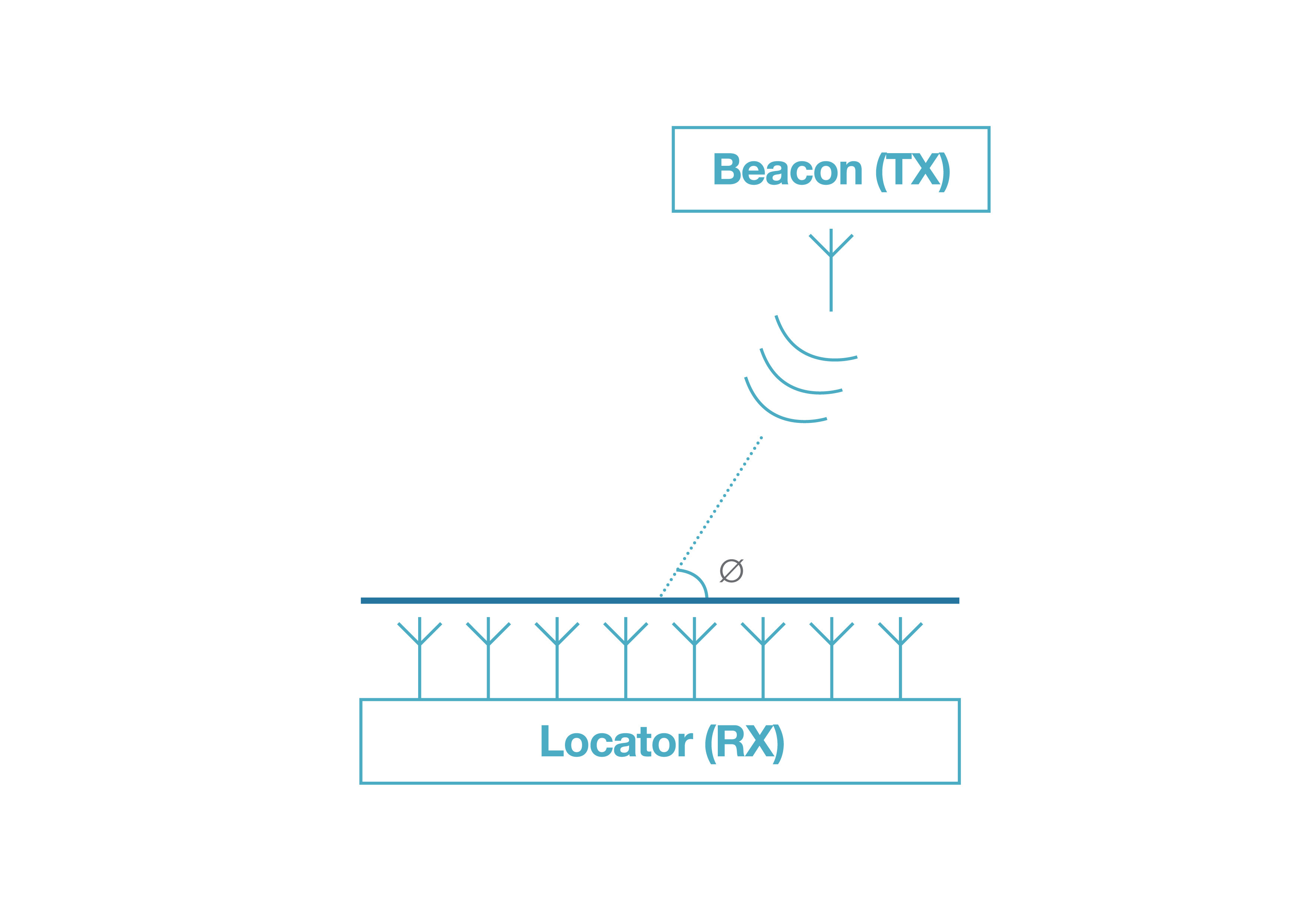
1. You can find the AoA with a multi-antenna linear array for a receiver and a device with one antenna for a transmitter.

In practice, the receiver device will need multiple ADC channels or use an RF switch to take samples from each channel. They’re called IQ-samples since a sample pair of In-phase and Quadrature-phase readings is taken from the same input signal. These samples have a 90-degree phase difference in the sampling. When this pair is considered to be a complex value, each value contains both phase and amplitude information and can be an input for the arrival angle estimation algorithm.

Radio waves travel at the speed of light (300,000 km/s). When using frequencies around 2.4 GHz, the corresponding wavelengths are about 0.125 m. The maximum distance between two adjacent antennas for most estimation algorithms is a half wavelength. Many algorithms require this; otherwise, we get effects similar to aliasing. There is no theoretical minimum distance limitation, but in practice, the minimum size is limited by the mechanical dimensions of the array plus, for example, mutual coupling between the antenna elements.

Measuring For AoD

The fundamental concept of measuring phase differences for AoD is the same as AoA, but device roles are swapped. In AoD, the device being tracked uses only one antenna, and the transmitter devices use multiple antennas (as seen in Fig. 2). The transmitter device sequentially switches the transmitting antenna, and the receiving side knows the antenna array configuration and switching sequence.

 

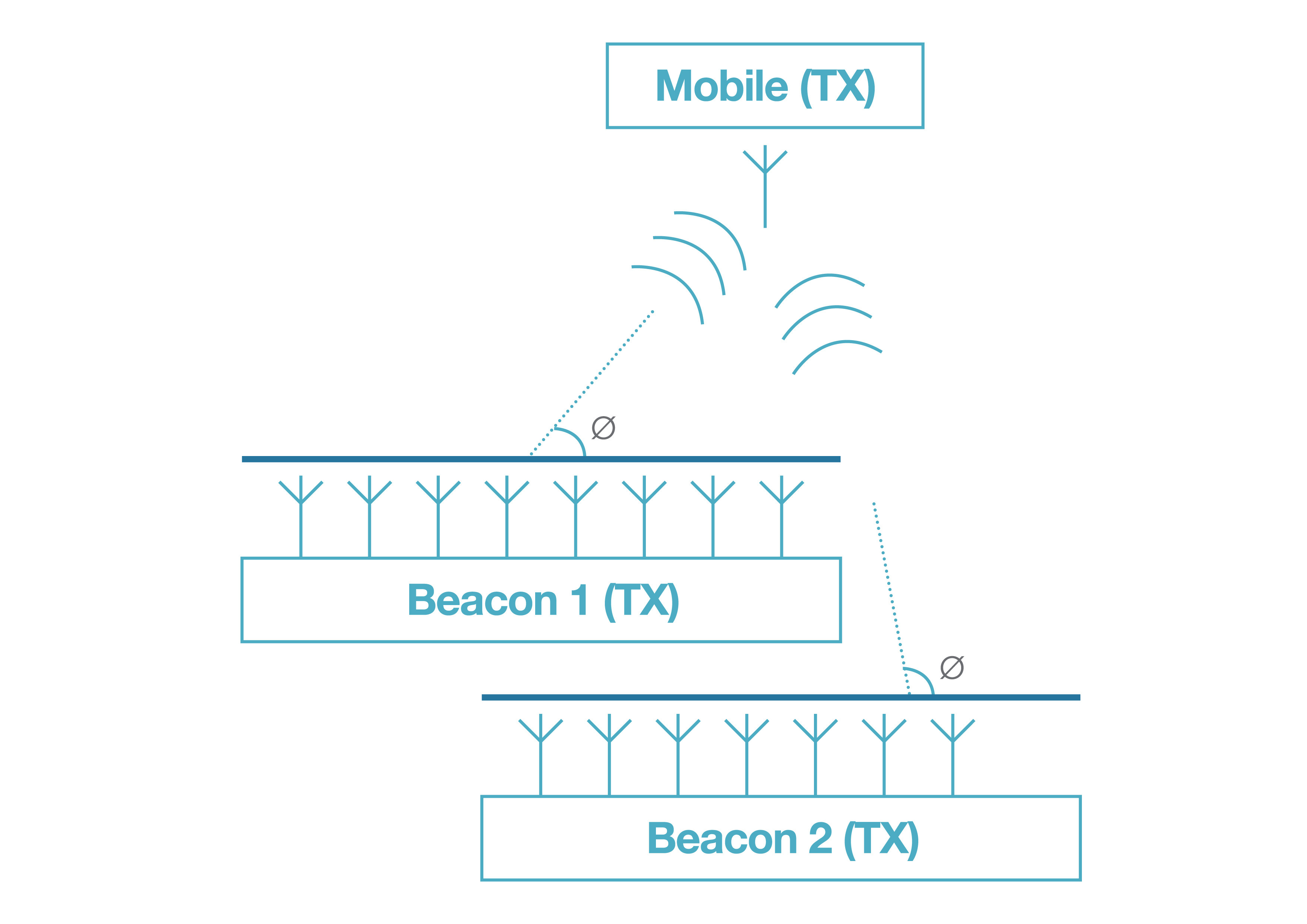
2. The AoD can be determined with a one-antenna linear array for a receiver and a device with multiple antenna for a transmitter.

When considering this from an application perspective, we can see a clear difference between these two techniques. In AoD, the receiving device can calculate its own position in space using angles from multiple beacons and their positions (by triangulation). In AoA, the receiving device tracks arrival angles for individual objects. Still, note that different combinations of these techniques can be performed so they don’t limit what can be done at the application level. In both Bluetooth AoA and AoD, the AoA/AoD-related control data is sent over a traditional data channel. Typically, these techniques can achieve a couple of degrees angular accuracy and around 0.5-m locationing accuracy, but these figures depend on the implementation of the locationing system.

Design Challenges

One of the biggest and perhaps most obvious challenges is determining how angle estimates are calculated based on the sample data. It’s not enough that we can calculate angle estimates in an ideal environment; we must also be able to calculate them in environments with very heavy multi-path in which signals are highly correlated or coherent. A coherent signal is one that’s a delayed and scaled version of some other signal. This can be the case when radio waves are reflected from walls, for example.

Other challenges include signal polarization. In most cases, we can’t control the mobile device’s polarization, so the system has to consider this. Also, signal noise, clock jitter, and signal propagation delays add their own variables to the problem. Depending on the system scale, the RAM and especially CPU requirements can be demanding for an embedded system. Many of the well-performing angle-estimation algorithms require a significant amount of processing power from the CPU.

As we cover some theory on antenna arrays and angle of arrival estimations, note that AoD can be derived from the AoA theory.

Angle of Arrival Theory

Angle estimation methods and antenna arrays are essential for the locationing system to work properly. The history of direction finding theory goes back more than 100 years when the first attempts to solve this problem used directional antennas and purely analog systems. Many years later, methods moved to the digital world, but the basic principles remain the same. These direction-finding methods are already used in many applications, such as medical equipment, and security and military devices. Let’s consider the basics of typical antenna arrays and estimation algorithms. Direction finding refers to the general problem of estimating arrival and departure angles.

Antenna Arrays

Antenna arrays for direction finding are usually divided into categories. The most common ones are uniform linear array (ULA), uniform rectangular array (URA), and uniform circular array (UCA). The linear array is one dimensional, meaning that all the antennas in the array lie on a single line, whereas the rectangular and circular arrays are two dimensional, meaning that the antennas are spread in two dimensions (on a plane). Using a one-dimensional array, one can reliably measure only the azimuth angle, assuming the tracked device moves consistently on the same plane. Furthermore, with two-dimensional arrays, one can reliably measure both azimuth and elevation angles in the 3D half-space. If the array is extended to a full 3D array (antennas spread on all three Cartesian coordinates), we can measure the full 3D space.

Designing an antenna array for direction finding is not a straightforward task. When antennas are placed in an array, they start affecting each other’s responses; this is called mutual coupling. Keep in mind that, in most cases, we can’t control the polarization of the transmitting end. This creates an additional challenge for the designer. In IoT applications, the devices are often expected to be small and even work in very high-frequency bands. Estimation algorithms often require certain properties from the array. For example, the estimation algorithm called ESPRIT works on the mathematical assumption that the array is divided into two identical subarrays.

Angle Estimation Algorithms

Let's look at the mathematical/algorithmic problem of estimating the arrival angle based on the input IQ-data. The problem definition itself is simple—estimate the arrival angle of an emitted (narrowband) signal arriving at the receiving array. While the problem statement sounds trivial, a robust, real-world solution for this problem is not easy and can require much processing power from the hardware.

Making MUSIC

Next, I’ll present an approach for solving this problem, a technique called multiple signal classification (MUSIC). While I won’t examine proofs of any theorems or reasons why this method works, I will give a high-level view of the algorithm, which is shown in Figure 3.

 

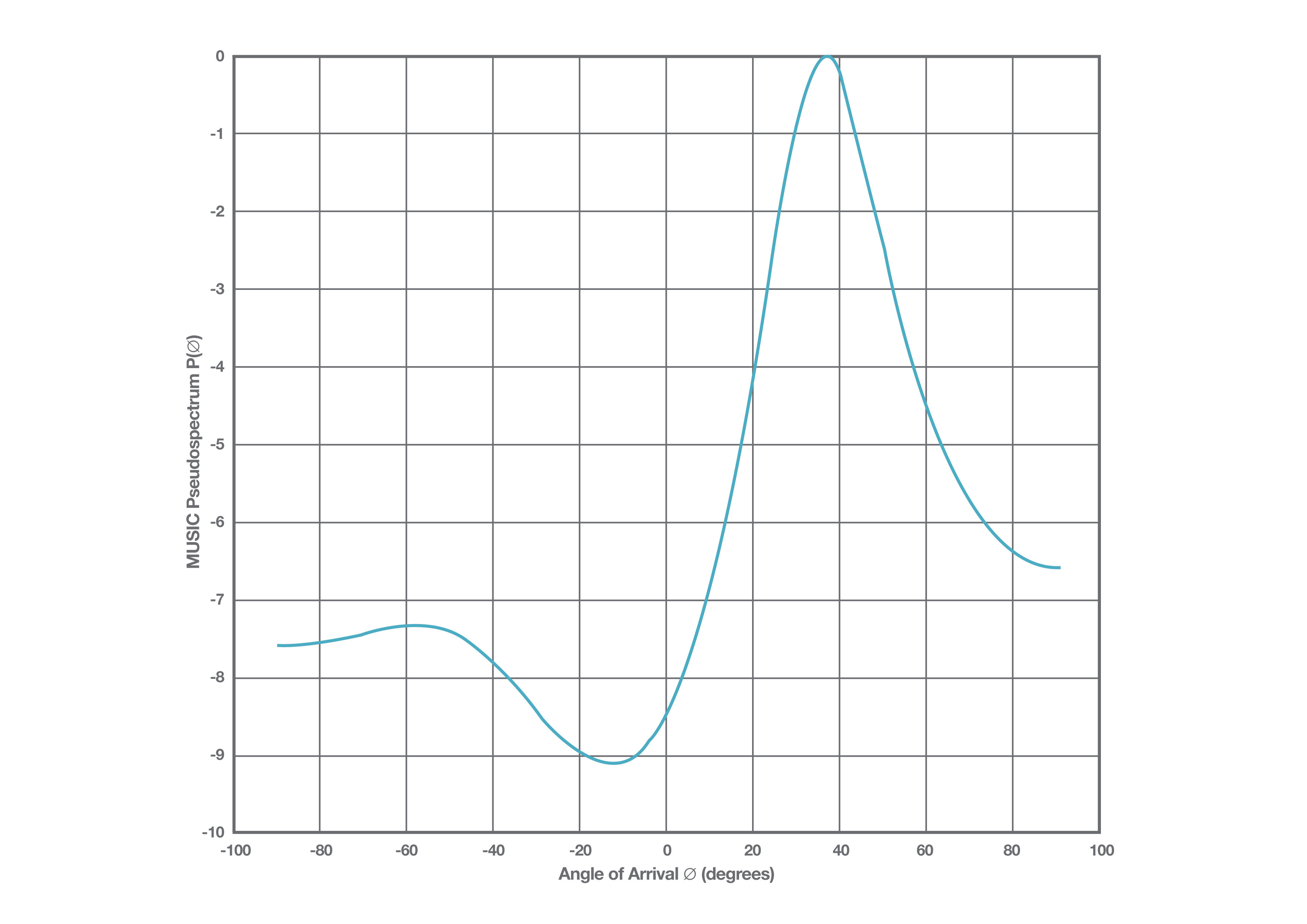
3. Pictured here is the MUSIC pseudospectrum for an eight-antenna ULA with a peak of 36.5 degrees.

Let's begin with a mathematical model of a uniform linear array. We’re given a data vector of IQ-samples for each antenna, which we’ll call x. Now, a phase shift is seen by each antenna (which can be 0) plus some noise, , in the measurements, so  can be written as a function of time :

x(t) = a(θ)s(t) + n(t) (1)

where  is the signal sent over the air, and  is the steering vector of the antenna array:

a(θ) = [1, e^{j2πdsin(θ)/λ}, …, e^{j2π(m-1)dsin(θ)/λ} (2)

where  is the distance between adjacent antennas,  is the signal’s wavelength;  is the number of elements in the antenna array, and  stands for the arrival angle.

Steering vector (2) describes how signals on each antenna are phase shifted because of the varying distances to the transmitter. Using equation (1), we can approximate the so-called sample covariance matrix, Rxx, by calculating

, (3)

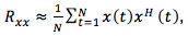
where H stands for the Hermitian transpose of a matrix.

The sample covariance matrix will be used as an input for the estimate algorithm. MUSIC direction of arrival estimation algorithm is also called the subspace estimator. The algorithm performs eigendecomposition on the covariance matrix :

R_xx = V AV^-1 (4)

where  is a diagonal matrix containing eigenvalues and containing the corresponding eigenvectors of R_XX.

Let’s now assume we’re trying to estimate the arrival angle for one transmitter with an  antenna linear array. It can be shown that the eigenvectors of  either belong to so-called noise or signal subspace. If the eigenvalues are sorted in ascending order, the corresponding  eigenvectors span the noise subspace, which is orthogonal to the signal subspace. Based on the orthogonality information, we can calculate the pseudo spectrum:

P:P(θ) = 1/a^H(θ)VV^Ha(θ) (5)

The final step is to loop through the desired values of  and find the maximum peak value of , which corresponds the angle of arrival (argument ) we wish to measure.

In an ideal case, MUSIC has very good resolution in a good signal-to-noise (SNR) environment and is very accurate. On the other hand, its performance isn’t very good when the input signals are highly correlated. This is the case especially in an indoor environment. Multipath effects distort the pseudo-spectrum causing it to have maximums at the wrong locations.

Spatial Smoothing

Spatial smoothing is a method for solving problems caused by multipathing (when coherent signals are present). It can be proven that the signal covariance matrix can be "decorrelated" by calculating an averaged covariance matrix using subarrays of the original covariance matrix. For a two-dimensional array, this can be written in the following manner:

 (6)

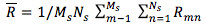
where  and  are the number of subarrays in x  and y directions respectively and  stands for the :th subarray covariance matrix.

The resulting covariance matrix can now be used as a decorrelated version of the covariance matrix and fed to the MUSIC algorithm to produce correct results. The downside of spatial smoothing is that it reduces the size of the covariance matrix, which further reduces the accuracy of the estimate.

Keep in mind that the Bluetooth AoA and AoD phase-based direction-finding systems require an antenna array, RF switches (or a multi-channel ADC), and sufficient processing power to run the estimation algorithms. Designing a proper antenna array and using an angle estimation algorithm are essential for an RTLS system. The RTLS designer should also keep in mind that high-performance estimator algorithms are often computationally demanding.

Sauli Lehtimäki is a Senior Software Engineer for Silicon Labs.

eletter-08-09-2018

eletter-08-07-2018